
Often people have asked me the difference between set_false_path, set_case_analysis and set_disable_timing. While the difference between these three is quite easy, it's the implications that leave many designers stumped.
Let me take a shot at explaining the difference.
1. FALSE PATH: All the timing paths which designers know won't be exercised on the fly, and they don't really need to meet any timing constraints on that path can be marked as false paths.
Tools would compute delays on all arcs on the false-path, would try to meet slopes/max-fanout/max-capacitance targets for all nodes along the path, but these paths would never surface up as timing (setup and hold) violations. However, if designers are too concerned about meeting slope and max cap targets, they usually prefer to mark such paths as set_multicycle_path instead.
Some examples of false path:

Consider the circuit above. The select line of the two multiplexers is complement of each other. STA tool, however, doesn't understand this logic and would treat all nodes as X (either 0 or 1). In practice, there can never be a timing path between
C -> E -> G
D -> F -> G
And these can be marked as false paths.
2. CASE ANALYSIS: Using set_case_analysis, any node can be constrained to a boolean logic value of 1 or 0. All case values are evaluated and propagated through the design. For example, if one input of an AND gate is 0, 0 being the controlling value, the output of AND gate would also be 0 and this 0 is propagated downstream. The timing arcs for set_case_analysis are not evaluated and they never show up in the timing reports. However, PnR tooks would still fix max transition, max capacitance and max-fanout violations on these nets/pins.
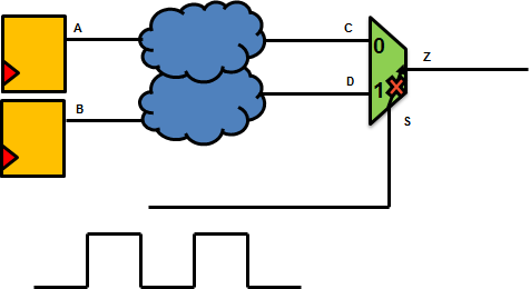
3. DISABLE TIMING: This disables a particular timing arc, and that timing arc or any timing path through the disabled timing arc is not computed. This tends to be a bit disruptive as compared to false paths or case analysis, but in some cases this is indispensable and the easiest way to achieve the intent. For example if you have a MUX based divider which receives the clock signal at the select line of the multiplexer, and two functional enables at the multiplexer inputs, STA tool would try to propagate the clock to the output of the MUX via the MUX select line to the output. But for a MUX, a select line only controls what gets propagated to the output. In practice, there's no arc between select and output and should be disabled.
Both case analysis and disable timing result in fewer timing paths to be analyzed. False path still tries to fix the design rule (max cap, max transition and max fanout) violations.
Tools would compute delays on all arcs on the false-path, would try to meet slopes/max-fanout/max-capacitance targets for all nodes along the path, but these paths would never surface up as timing (setup and hold) violations. However, if designers are too concerned about meeting slope and max cap targets, they usually prefer to mark such paths as set_multicycle_path instead.
Some examples of false path:

Consider the circuit above. The select line of the two multiplexers is complement of each other. STA tool, however, doesn't understand this logic and would treat all nodes as X (either 0 or 1). In practice, there can never be a timing path between
C -> E -> G
D -> F -> G
And these can be marked as false paths.
2. CASE ANALYSIS: Using set_case_analysis, any node can be constrained to a boolean logic value of 1 or 0. All case values are evaluated and propagated through the design. For example, if one input of an AND gate is 0, 0 being the controlling value, the output of AND gate would also be 0 and this 0 is propagated downstream. The timing arcs for set_case_analysis are not evaluated and they never show up in the timing reports. However, PnR tooks would still fix max transition, max capacitance and max-fanout violations on these nets/pins.
- Some latest tool versions also support a case value of static which means that the node will always be static (never toggle), and this is used to reduce the pessimism which doing noise analysis.
- Case analysis is also particularly useful for DFT modes where you would want to set a few configuration registers and drive the chip into a particular DFT mode: like atspeed, shift or stuck-at mode. This acts as an additional level of verification because you'd expect to see only scan chains in the shift mode with scan enable being 1. You'd expect to see functional paths in the atspeed mode with scan enable being X, and you'd expect to see only paths ending at functional register inputs in the stuck-at mode with scan enable being 0.
3. DISABLE TIMING: This disables a particular timing arc, and that timing arc or any timing path through the disabled timing arc is not computed. This tends to be a bit disruptive as compared to false paths or case analysis, but in some cases this is indispensable and the easiest way to achieve the intent. For example if you have a MUX based divider which receives the clock signal at the select line of the multiplexer, and two functional enables at the multiplexer inputs, STA tool would try to propagate the clock to the output of the MUX via the MUX select line to the output. But for a MUX, a select line only controls what gets propagated to the output. In practice, there's no arc between select and output and should be disabled.
Both case analysis and disable timing result in fewer timing paths to be analyzed. False path still tries to fix the design rule (max cap, max transition and max fanout) violations.


